Getting Started with AstroPath in SciServer

AstroPath is an interdisplinary intiative that adapts tools from the Sloan Digital Sky Survey (SDSS) to generate high-fidelity, whole-slide spatial maps of the tumor microenvironment (TME). By leveraging multispectral imaging and treating cells like stars or galaxies, AstroPath profiles 100,000–2 million cells per slide, offering an unprecedented single-cell view of tumors. For more information about what the datasets contain, see SciServer’s Biomedical datasets page. 

Should you need additional help or further information during or after the tutorial, see How to Use SciServer in the SciServer Help pages.

Create a SciServer Account and Join the AstroPath science domain 

If you haven’t already, head over to the SciServer website and create a new username and password. Detailed directions on creating an account can be found in the How to use SciServer guide. This guide also contains important additional information and resources for understanding the SciServer. 

Next, to obtain access to the AstroPath datasets, join the SciServer AstroPath science domain.  

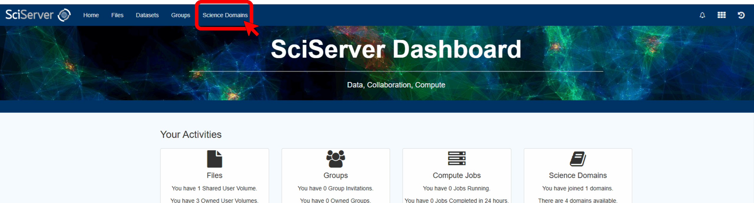
To do this, first log in to SciServer with your new account. Then, from the SciServer Dashboard, click “Science Domains” located in the top menu bar.

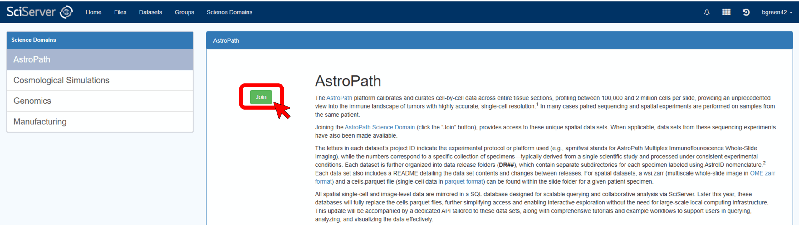
Select “AstroPath” from the list in the left panel and click the green “Join” button in the main panel.

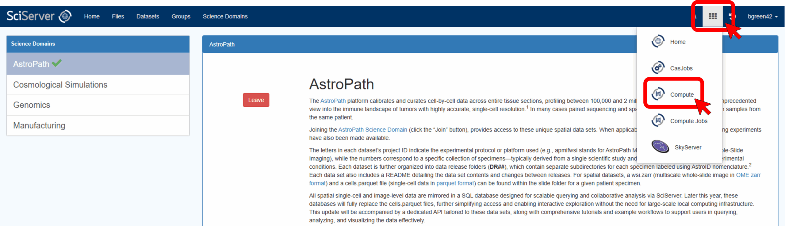
And that’s it, you should now have access to the AstroPath datasets! To start analyzing the data you can either use SciServer Compute or SciServer’s CasJobs API.  

SciServer Compute is an “application that allows users to easily create and run Jupyter Notebooks containing code and instructions to analyze and process SciServer hosted data sets.” More details about these compute environments can be found in the documentation. 

Simply put, SciServer Compute provides a cloud computing environment with some preinstalled software (such as Jupyter or R) so that you can jump right into accessing the datasets without having to install anything on your computer. 

A brief example using SciServer Compute can be found below. SciServer also offers some example notebooks. For more details on SciServer’s CasJobs API see the API Documentation. 

Create a SciServer Compute Container

To start analyzing the AstroPath data, create a container and include the AstroPath datasets.

Start by clicking on the tools icon in the top left of the SciServer Dashboard and select Compute.

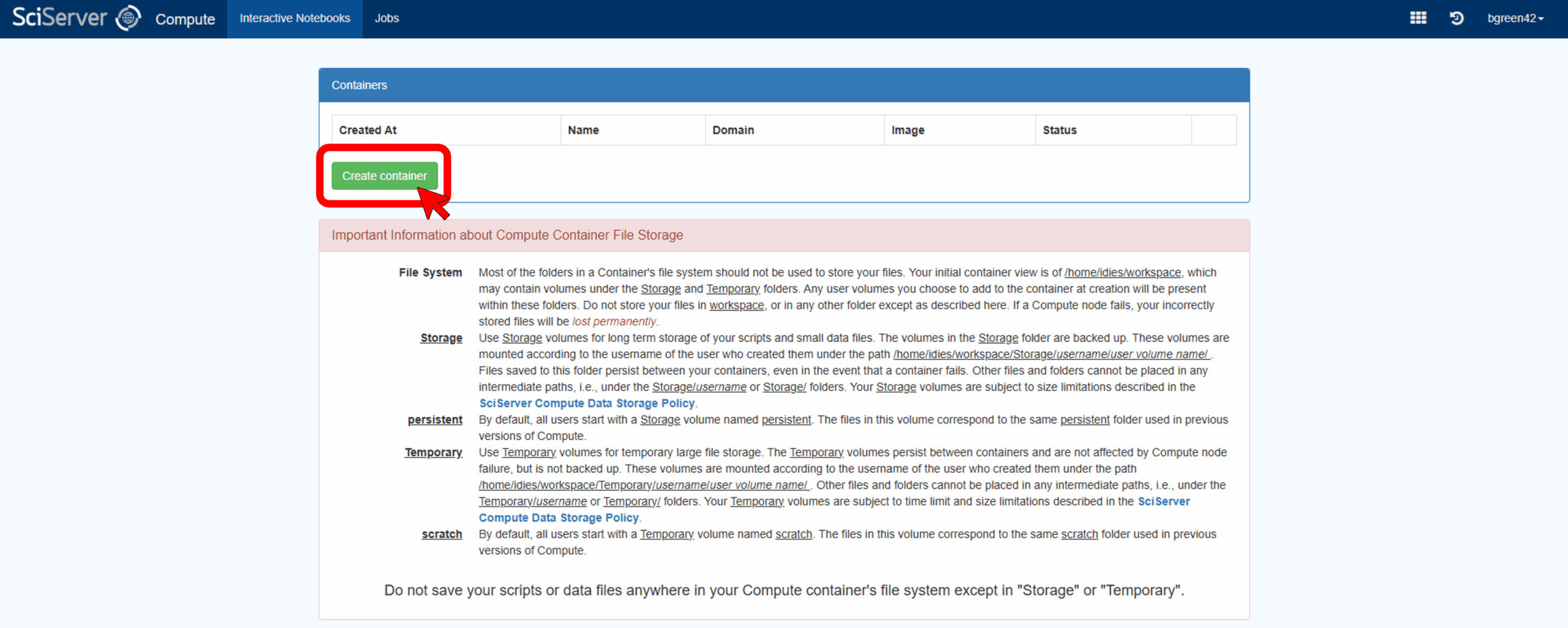
Before creating a container, please take a moment to note the information regarding file storage at the bottom of the Compute page. These details may not make perfect sense now but will become important in the future. Essentially, you have access to a few different folders in the container, but when and how long files will exist may change over time depending on where it is saved.

Next, click on “Create Container.”

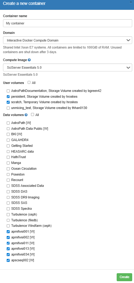
A window will open with options for how to initialize the container – see the image below for an example of what it may look like. In this window, give the container a unique name under Container name and leave the Domain option as it is. For the Compute Image use SciServer Essentials 3.0. Under Data Volumes, select the datasets you want access to. The AstroPath volumes all start with “ap” (e.g. “apmifwsi002”, “apmifwsi011”, etc). Finally click Create in the lower right-hand corner. 

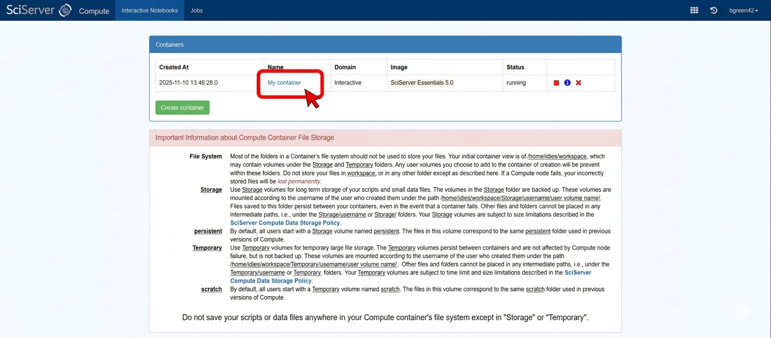
Once you create the container, you will be returned to the Compute page and see its name in the list. To activate the container click on its name in the table of containers. This should open a new window for the container with a JupyterLab interface.

Use JupyterLab

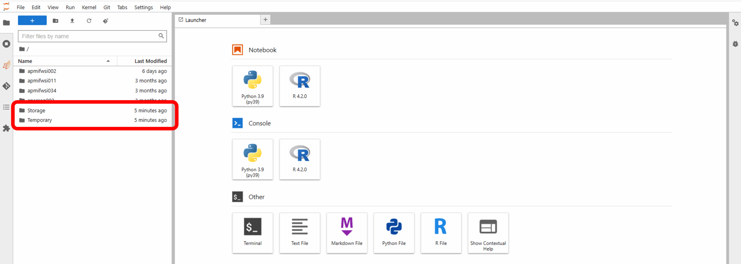
On the left side of the screen, you will see the data volumes you selected in the “Create container” window. You can navigate through the directory structure to examine the data. You will not be able to create any files in these directories, as they are read-only.

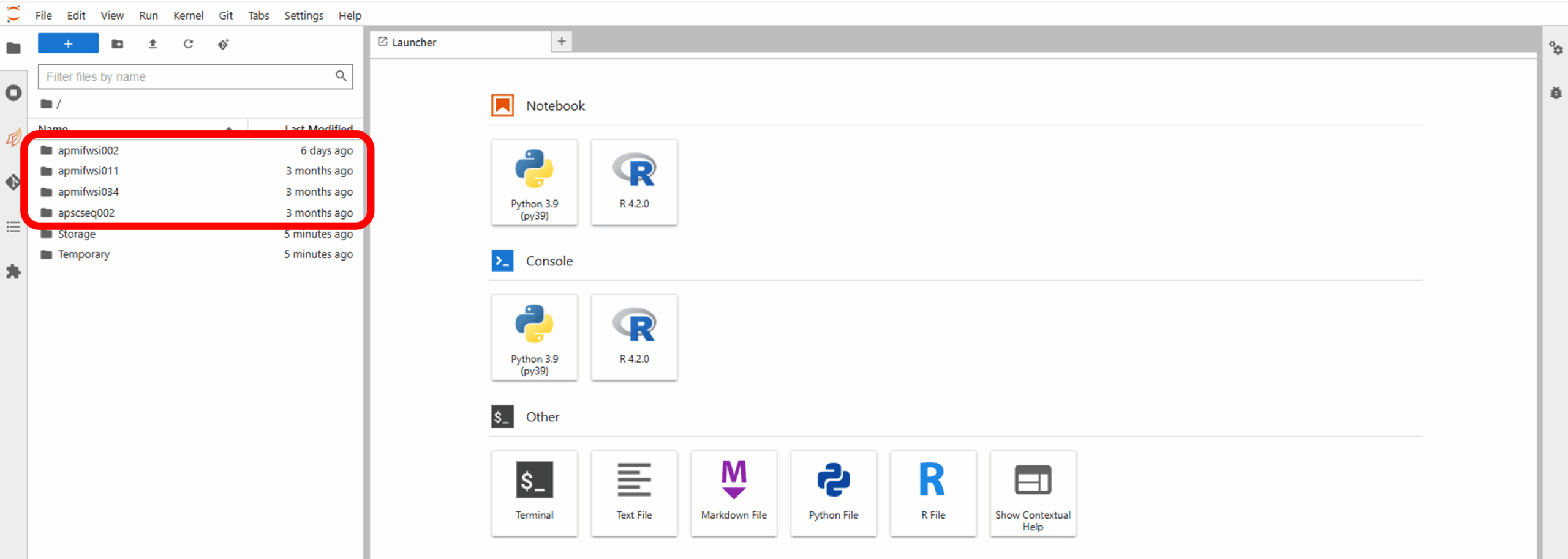
Navigate back to the home directory and go into “Storage” or “Temporary”. These folders persist between containers you create and are recommended for analysis work. “Storage” is backed up, while “Temporary” is not and unused files may be deleted.

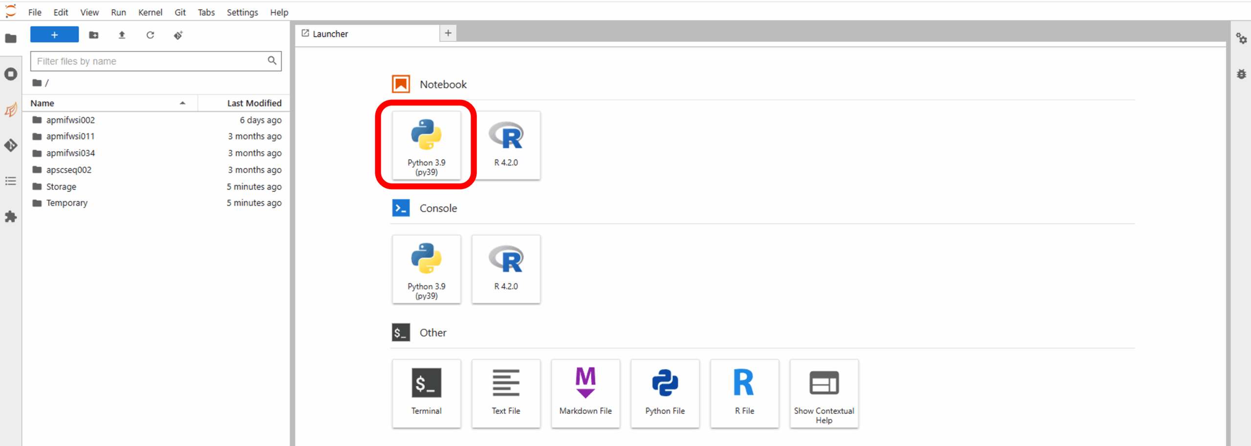
You can open a Jupyter notebook via the buttons on the right side of the screen and analyze the data in Jupyter.

The root of the file system accessible from your container is /home/idies/workspace/. The data will be in, for example, /home/idies/workspace/apmifwsi002/.

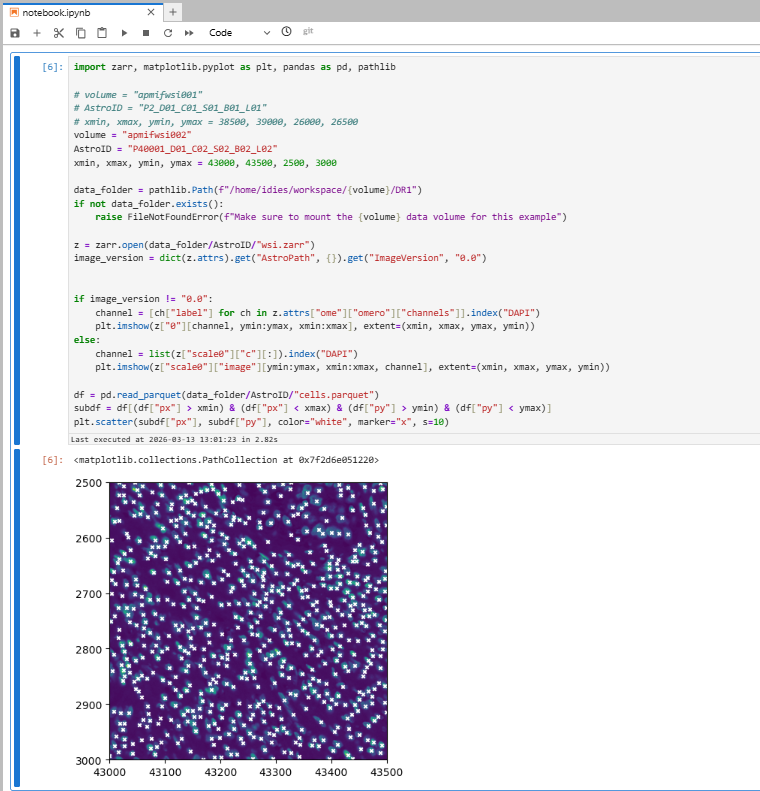
Below is a minimal example of code from a Jupyter notebook to show a small area of the slide image, with each cells marked with an “x”. You can paste it directly into your notebook. This example requires selecting the apmifwsi002 volume at the time of container creation. The screenshot below shows the expected output.

import zarr, matplotlib.pyplot as plt, pandas as pd, pathlib 

data_folder = pathlib.Path("/home/idies/workspace/apmifwsi002/DR1/P40001_D01_C02_S02_B02_L02") 

if not data_folder.exists(): raise FileNotFoundError("Make sure to mount the apmifwsi002 data volume for this example") 

z = zarr.open(data_folder/"wsi.zarr") 

xmin, xmax, ymin, ymax = 43000, 43500, 2500, 3000 

plt.imshow(z["scale0"].image[ymin:ymax,xmin:xmax,0], extent=(xmin, xmax, ymax, ymin)) 

df = pd.read_parquet(data_folder/"cells.parquet") 

subdf = df[(df["px"] > xmin) & (df["px"] < xmax) & (df["py"] > ymin) & (df["py"] < ymax)] 

plt.scatter(subdf["px"], subdf["py"], color="white", marker="x", s=10)